Getting started

Getting started

1a. Installation using pre-built libraries

The easiest way to install the package is:

julia> ]
(@v1.6) pkg> add PETSc

which will install a pre-built PETSc library (PETSc_jll) as well as MPI.jl on your system. This will work both in serial and in parallel on your machine.

1b. Installation using pre-built libraries

On many high-performance clusters, you will have to use the provided MPI installation for that cluster and the default download above will not be sufficient. Alternatively, you may be interested in a PETSc installation that comes with additional external packages. Ensure that this PETSc installation is compiled as a dynamic (and not a static) library, after which you need to set the environmental variable JULIA_PETSC_LIBRARY to link to your PETSc installation:

$export JULIA_PETSC_LIBRARY = /path/to/your/petsc/installation:

Now rebuild the package:

julia> ]
pkg> build PETSc

2. Solving a linear system of equations

Lets consider the following elliptic equation:

\[\begin{aligned} {\partial^2 T \over \partial x^2} = 0, T(0) = 1, T(1) = 11 \end{aligned}\]

julia> using PETSc
julia> petsclib = PETSc.petsclibs[1]
julia> PETSc.initialize(petsclib)
julia> n   =  11
julia> Δx  =  1. / (n - 1)

Let's first define the matrix with coefficients:

julia> nnz =  ones(Int64,n); nnz[2:n-1] .= 3;
julia> A   =  PETSc.MatSeqAIJ{Float64}(n,n,nnz);
julia> for i=2:n-1
            A[i,i-1] =  1/Δx^2
            A[i,i  ] = -2/Δx^2
            A[i,i+1] =  1/Δx^2
       end
       A[1,1]=1; A[n,n]=1;
julia> PETSc.assemble(A)
julia> A
Mat Object: 1 MPI processes
  type: seqaij
row 0: (0, 1.) 
row 1: (0, 100.)  (1, -200.)  (2, 100.) 
row 2: (1, 100.)  (2, -200.)  (3, 100.) 
row 3: (2, 100.)  (3, -200.)  (4, 100.) 
row 4: (3, 100.)  (4, -200.)  (5, 100.) 
row 5: (4, 100.)  (5, -200.)  (6, 100.) 
row 6: (5, 100.)  (6, -200.)  (7, 100.) 
row 7: (6, 100.)  (7, -200.)  (8, 100.) 
row 8: (7, 100.)  (8, -200.)  (9, 100.) 
row 9: (8, 100.)  (9, -200.)  (10, 100.) 
row 10: (10, 1.)

Now, lets define the right-hand-size vector rhs as a julia vector:

julia> rhs = zeros(n); rhs[1]=1; rhs[11]=11;

Next, we define the linear solver for the matrix A, which is done by setting a KSP solver:

julia> ksp = PETSc.KSP(A; ksp_rtol=1e-8, pc_type="jacobi", ksp_monitor=true)

Note that you can specify all PETSc command-line options as keywords here.

Solving the system of equations is simple:

julia> sol = ksp\rhs
  0 KSP Residual norm 1.104536101719e+01 
  1 KSP Residual norm 4.939635614091e+00 
  2 KSP Residual norm 2.410295378065e+00 
  3 KSP Residual norm 1.462993806273e+00 
  4 KSP Residual norm 1.004123728835e+00 
  5 KSP Residual norm 7.700861485629e-01 
  6 KSP Residual norm 6.165623662013e-01 
  7 KSP Residual norm 4.972507567923e-01 
  8 KSP Residual norm 4.074986825669e-01 
  9 KSP Residual norm 3.398492183940e-01 
 10 KSP Residual norm 3.283015493450e-15 
11-element Vector{Float64}:
  1.0
  2.000000000000001
  3.0000000000000013
  4.000000000000001
  5.000000000000002
  6.0
  7.0000000000000036
  8.000000000000002
  9.000000000000004
 10.000000000000002
 11.0

And since we are using julia, plotting the solution can be done with

julia> using Plots
julia> plot(0:Δx:1,sol, ylabel="solution",xlabel="x")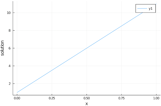

linear_solution

3. Nonlinear example

Let's solve the coupled system of nonlinear equations:

\[\begin{aligned} x^2 + x y &= 3 \\ x y + y^2 &= 6 \end{aligned}\]

for $x$ and $y$, which can be written in terms of a residual vector $f$:

\[f = \binom{ x^2 + x y - 3} {x y + y^2 - 6}\]

In order to solve this, we need to provide a residual function that computes $f$:

julia> function F!(cfx, cx, args...)
         x     = PETSc.unsafe_localarray(Float64, cx;  write=false)   # read array
         fx    = PETSc.unsafe_localarray(Float64, cfx; read=false)    # write array
         
         fx[1] = x[1]^2 + x[1]*x[2] - 3
         fx[2] = x[1]*x[2] + x[2]^2 - 6
         
          Base.finalize(fx)
          Base.finalize(x)
       end

In addition, we need to provide the Jacobian:

\[J = \begin{pmatrix} \frac{\partial f_1}{ \partial x} & \frac{\partial f_1}{ \partial y} \\ \frac{\partial f_2}{ \partial x} & \frac{\partial f_2}{ \partial y} \\ \end{pmatrix} = \begin{pmatrix} 2x + y & x \\ y & x + 2y \\ \end{pmatrix}\]

In Julia, this is:

julia> function updateJ!(cx, J, args...)
            x      = PETSc.unsafe_localarray(Float64, cx;  write=false)
            J[1,1] = 2x[1] + x[2]
            J[1,2] = x[1]
            J[2,1] = x[2]
            J[2,2] = x[1] + 2x[2]
            Base.finalize(x)
            PETSc.assemble(J)          
        end

In order to solve this using the PETSc nonlinear equation solvers, you first define the SNES solver together with the jacobian and residual functions as

julia> using PETSc, MPI
julia> S = PETSc.SNES{Float64}(petsclib,MPI.COMM_SELF; ksp_rtol=1e-4, pc_type="none")
julia> PETSc.setfunction!(S, F!, PETSc.VecSeq(zeros(2)))
julia> J = zeros(2,2)
julia> PJ = PETSc.MatSeqDense(J)
julia> PETSc.setjacobian!(S, updateJ!, PJ, PJ)

You can solve this as:

julia> PETSc.solve!([2.0,3.0], S)
2-element Vector{Float64}:
 1.000000003259629
 1.999999998137355

which indeed recovers the analytical solution $(x=1, y=2)$.